Book Tour

This page provides a brief overview of the overall flow of the book. Elsewhere on the site, you may find a detailed table of contents, examples of specific chapters, and examples of specific programming exercises. The figures on this page are taken from the 150+ figures in the book, with each figure number indicating the corresponding figure in the book.

Figure 1.1: Motivating example.

In Chapter 1: Why Geometric Algebra?, we introduce the capabilities of geometric algebra with a motivating example (see Figure 1.1). The example reveals its main characteristics for computations in Euclidean geometry: the convenient construction of extended objects such as circles; of operators like rotation around an axis or reflection in a mirror; the universality of geometric operators on all elements; and the easy interpolation procedure. We show how a GA-based computer program looks, and explain the structure of the book. This chapter can be viewed here in its entirety.

Part I: GEOMETRIC ALGEBRA

Part I introduces the basics of geometric algebra. It provides the algebraic structure, with products inspired by the desire to represent linear subspaces and geometric operations on them. Throughout, the concepts are illustrated and developed through drills, structural exercises, and programming exercises.

Figure 2.3: The outer product.

To extend the representational capabilities of linear algebra, Chapter 2: Spanning Oriented Subspaces introduces the outer product. The outer product of two vectors is algebraically a 2-blade. In its most simple geometric interpretation such a 2-blade represents the 2-dimensional subspace through the origin, spanned by the vectors, as shown in Figure 2.3 (left). An outer product of three vectors is a 3-blade, see Figure 2.3 (right). A 3-blade represents the volume spanned by the three vectors. Such extended geometrical entities are now basic elements of algebraic computation.
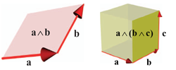
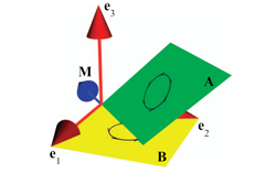
We use the blades of a geometric algebra to algebraically represent all geometrical primitives. The scalars in a vector space are represented as 0-blades, the vectors by 1-blades, and the oriented area elements are 2-blades. In Part II, we will give enriched interpretations to these blades. For example, in the homogeneous model 2-blades are used to represent lines and 3-blades represent planes; in the conformal model 3-blades represent circles, and so on.

Figure 3.3: The left contraction.

In Chapter 3: Metric Products of Subspaces, we generalize the dot product from linear algebra such that it is applicable to blades. These metric products allow us to measure angles and contents, orthogonalize vectors, perform projections, and so on. In figure 3.3, we depict the left contraction of a vector x and a 2-blade B, resulting in a vector which is contained in B, and perpendicular to x. It is an elementary construction, more fundamental than projection because it is linear in both x and B.
In this chapter, we also introduce dualization. Any element in geometric algebra has a dual representation, through its inner product relative to the total volume element of the space. Those 'geometrical complements' are often very convenient in computational expressions.

Figure 4.1b: Extending a linear transformation to blades.

Chapter 4: Linear Transformations of Subspaces shows that the usual linear transformations defined on vectors (1-blades) can be applied to k-blades, using the same formula. This enriches the descriptive and computational power of linear algebra considerably, since you can now apply linear transformations immediately to subspaces, without needing to decompose those into vectors first.
These linear transformations preserve the properties of the outer product, and are hence called outermorphisms. This chapter is a bit algebraic, but it is important to know how the subspace products transform under linear transformations.

Figure 5.2: The meet of two 2-blades.

In Chapter 5: Intersections and Unions of Subspaces, we codify those geometric operations algebraically, as the meet and join products of blades. They are algebraically a bit involved, and algorithmically somewhat expensive. Yet their geometric importance warrants the effort to generalize them: the algebraic ability to compute the common blade of two arbitrary blades translates (in Part II) as the geometric capability to intersect lines, planes, circles, spheres, etc. This chapter is somewhat abstract, and can be skimmed at first reading.

Figure 6.2: Ratios of vectors.

In Chapter 6: The Fundamental Product of Geometric Algebra, the magic of geometric algebra really begins to show. While the subspace products in the previous chapters are reasonably well known under the guise of 'multilinear algebra' (though often in cumbersome notations like tensors), the geometric product is unique to geometric algebra. It is surprisingly simple algebraically - being linear, associative, and giving scalar squares for vectors defines it fully. In this chapter, we carefully relate it to the outer product and contraction of the earlier chapters, to provide some geometric intuition for its structure and use.
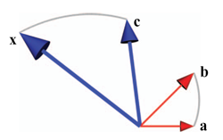
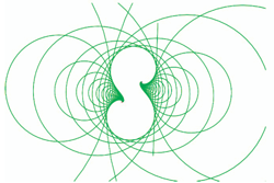
The geometric product is invertible, and this immediately simplifies the algebraic specification of a specific geometrical situation. You can divide by vectors, and in the planar example of Figure 6.2, you can use this capability to solve the equation x/c = b/a immediately as x = (b/a)c. Therefore the vector ratio (b/a) defines an operator that rotates and scales.

Figure 7.2: A rotation is a double reflection. It can be represented as the versor (b/a) which is the geometric product of two vectors which specify the rotation plane and half the rotation angle.

Chapter 7: Orthogonal Transformations as Versors describes how the most important generic use of the geometric product is by 'sandwiching' an object X to be transformed between a versor V and its inverse: X -> V X /V.
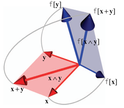
This is a universal, structure-preserving representation of the action of an operator onto any element: The transform of a geometric combination of elements equals the combination of the transforms of the elements. Any framework for geometry should obey this; what is nice about geometric algebra (used properly) is that it has this structure preservation inherently built in: its operators have this property, so no computational effort is required to make it true. (Actually, only orthogonal transformations have this desirable property; but in Part II we show techniques to ensure that important geometrical transformations become orthogonal in their representing algebra.)
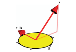
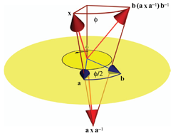
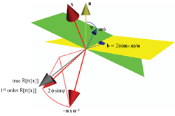
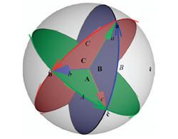
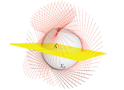
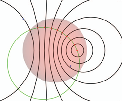
The most basic versor is a vector v, and the associated transformation a reflection in the plane perpendicular to v. Multiple applications of such versors then generates rotation versors, a.k.a. rotors, see Figure 7.2. These have all the properties of complex numbers and quaternions, but now in n-D and universally applicable in a real vector space context.

Figure 8.2: As a mirror rotates slightly, its reflections move. By a first order approximation in geometric differentiation, we easily find the locally circular orbit of a caustic.

Chapter 8: Geometric Differentiation is about the process of computing with small changes in geometric quantities. When the changes are small, those computations can be linear to a good approximation, and it is not too hard to develop a calculus for geometry by analogy to classical analysis.
When formulated with geometric algebra, it becomes possible to differentiate not only with respect to a scalar (as in real calculus) or a vector (as in vector calculus), but also with respect to general multivectors and k-blades. The differentiation operators follow the rules of geometric algebra: they are themselves elements to differentiate dependencies, but must use the non-commutative geometric product in their multiplication when applied to other elements. As you might expect, this has precisely the right geometric consequences for the differentiation process to give geometrically significant results.
In this book, we only give the basic principles, to allow you to interface with other texts that contain a more complete differential geometry in the GA formulation.

Part II: MODELS OF GEOMETRIES

Chapter 9: Modeling Geometries introduces the procedure of Part II: we will use the structure of geometric algebra introduced in Part I to model different aspects of geometry. As we do so, we are able to apply it to specific situations, permitting increasingly useful programming exercises.

Figure 10.3: Spherical geometry.

Chapter 10: The Vector Space Model - The Algebra of Directions is the first geometric model, and the most direct visualization of the structure of geometric algebra. All of Part I was in fact about characterizing k-dimensional directions. We develop that correspondence in more detail for a Euclidean space. This leads naturally to applications like: triangular equalities, spherical geometry, crystallographic point groups, interpolation and estimation of rotations. The latter is naturally performed by employing the 'logarithm of a rotor'. In all of those applications, the geometric product immensely simplifies the expression and derivation of advanced results.

Figure 11.2b: Lines as 2-blades in the homogeneous model.

Chapter 11: The Homogeneous Model embeds the familiar homogeneous coordinates used throughout computer graphics, robotics and computer vision into geometric algebra. This clarifies and extends its algebraic structure. Its basic elements are offset flats in Euclidean space, and these are the blades of its geometric algebra.
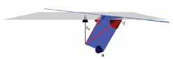
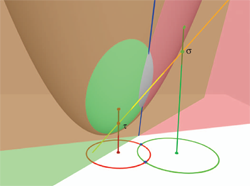
The outer product between two 1-blades representing geometric points is the 2-blade that represents the geometric line between those points (see Figure 11.2b). Naturally equivalent representations of the same geometry (such as by a point and a direction vector) become algebraically identical elements.
The homogeneous model connects well to existing software for computer graphics and computer vision, and we demonstrate that by the programming examples of this chapter.

Figure 12.4: A pinhole camera with a plane of rays.

Chapter 12: Applications of the Homogeneous Model treats two obvious uses of the homogeneous model for non-metric applications: the intersection of flats, and projective imaging by cameras.
Classically, the former is treated by Plücker coordinates, which then seem like a separate and non-intuitive trick; we show what they actually are, and how the algebra of the homogeneous model empowers the user to span and intersect flats generically.
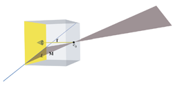
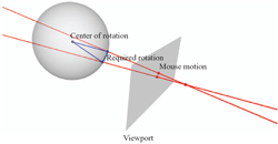
Imaging by (multiple) cameras in its usual treatment gets obscured by the need to represent the relevant operations in coordinate form; here, too, the homogeneous model provides algebraic insight into the straightforward essence of the geometry-based techniques.

Figure 13.4: Screw representation of rigid body motions in the conformal model.

Chapter 13: The Conformal Model - Operational Euclidean Geometry is the central chapter of the book. It applies the modeling principles to design an algebra that is automatically structure-preserving for the constructions of n-dimensional Euclidean geometry. This conformal model is the geometric algebra of a representational space with two extra dimensions. One dimension represents the point at the origin (as in the homogeneous model) and the other the unique point at infinity. These are null dimensions, contributing to the metric properties in a subtle but convenient way.

Figure 13.7: Differentiation of a reflected line in a rotating mirror.

The defining property of the conformal model is that the inner product between 1-blades represents the squared distance between Euclidean points. This guarantees that Euclidean motion are represented by orthogonal transformations. Those are coded as versors, and that results in the structure-preservation. The logarithm of a rigid body motion can then be derived in closed form, permitting screw-like interpolation of such motions (Figure 13.4), and their structure preserving differentiation (Figure 13.7).

Figure 14.6: The Euclidean intersection of circles computed as the meet of representing planes.

In Chapter 14: New Primitives for Euclidean Geometry, we show that the blades of the conformal model can represent an algebraically consistent catalog of elements that are useful in Euclidean geometry. They give us spheres, circles, point pairs and tangents as direct elements of computation. We carefully develop the representation of these new elements and show how to retrieve their parameters. You will for instance see that the sphere through the four points p, q, r and s, is the blade p^q^r^s, and that you can immediately read off its center and radius from the dual blade.
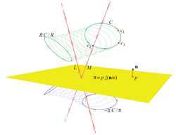
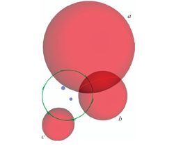
We also give the geometry behind the algebra of the conformal model, and show in detail how the universal meet of flat subspaces can perform the intersection of circles and spheres.

Figure 15.1b: The meet and plunge of spheres.

Chapter 15: Constructions in Euclidean Geometry. The algebraically consistent structure provides universal constructions in Euclidean geometry. Some of those are unusual, but useful: there is for example a simple expression for the element perpendicularly intersecting other elements (the plunge of Figure 15.1b), and how to compute the tangent to a basic element (circle, sphere, plane) without differentiation.
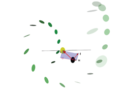
We show how all the various concepts of a 'vector' in classical geometry now have found their specific expression in the conformal model. Normal vector, position vector, free vector, line vector and tangent vector now all automatically move in the correct way under the same Euclidean versors. This demonstrates clearly that the conformal model performs both the geometrical computations and the 'data type management' required in Euclidean geometry.

Figure 16.6a: Circles transformed conformally.

Even with all the new techniques for Euclidean geometry of the previous three chapters, the possibilities of the conformal model are not exhausted. In Chapter 16: Conformal Operators we show that the versor of the conformal model represent conformal transformations that preserve angles (Figure 16.6a). These include reflection in a sphere, and uniform scaling; Euclidean motions were just a special case. The fact that the general conformal transformations can be represented as versors finally explains the name of the 'conformal' model.

Figure 16.13f: Hyperbolic geometry.

The non-Euclidean hyperbolic and elliptic geometries can now also be processed in the same model (Figure 16.3f), merely by introducing another conformal 1-blade to represent the associated concept of 'infinity'.

Chapter 17: Operational Models for Geometries sums up the principles that guided the design of structure preserving models in Part II, and makes an inventory of geometries for which we know such operational models. More will presumably be found, all obeying the same design principles - the conformal model is merely the first.

Part III: IMPLEMENTING GEOMETRIC ALGEBRA

To use geometric algebra as an actual specification of efficient code in geometric applications, you need to think carefully about its implementation. The conformal model of a 3D Euclidean space uses a 32-dimensional geometric algebra, and a naive implementation would be prohibitively slow. In this Part III, we show that you can use the structure and sparseness of geometric algebra to compete in efficiency with the usual, coordinate-based, hand-coded minimal solutions for applications such as ray-tracing. The coordinate-free specifications in the geometric algebra code then truly acts like a high-level programming language for geometry.

We make an inventory of the issues in Chapter 18: Implementation Issues, focusing on the various levels of the algebraic structure in a typical application. Each of those levels is subsequently treated in a separate chapter. (We also briefly mention alternatives to our preferred approach, and why they are in general inferior.)

In Chapter 19: Basis Blades and Operations we encode the elements of the additive basis for blades efficiently in a bitmap and give algorithms for the basis products of such basis elements.

Chapter 20: The Linear Products and Operations then gives two methods to compose the linear products (outer product, contractions and geometric product) from the results on basis blades. The mathematically pure use of the linear algebra structure of geometric algebra (as a Clifford algebra) in a matrix implementation is just not good enough; processing a 'list of basis blades' is more efficient.

In Chapter 21: Fundamental Algorithms for Nonlinear Products, we process the more awkward operations of geometric algebra, such as inverses and the meet and join products. This involves giving algorithms for factorization (both in terms of outer product and geometric product), for testing whether a multivector is a blade or versor, and more such elementary capabilities.

In Chapter 22: Specializing the Structure for Efficiency, we discuss in detail how we used generative programming techniques to construct our own software Gaigen2. It enables using geometric algebra at the high-level for the specification of geometrical operations, and uses its structure in a code generator to produce low-level coordinate operations with an efficiency similar to the best classical solutions. This is demonstrated by some benchmark experiments.

Figure 23.3: The design of a GA-based user interface.

Chapter 23: Using the Geometry in a Ray-Tracing Application works through an application in considerable detail. We show how to weigh the various representational possibilities offered by the conformal model to choose the most efficient structured representation for this application. As an aside, we show how to build a graphical user interface, using mouse interactions to build the corresponding versors in a coordinate-free manner.

Appendices, References and Index

The book contains appendices giving the detailed proofs of some important statements, and a convenient overview of the more useful definitions and formulas. Each Chapter ends with a 'Further Reading' section, relating its contents to the most relevant literature provided in the References. A 14-page index helps you to navigate the book effectively.